

Inspection systems for 3D printing have usually arrived after the damage is done. A part finishes printing, comes off the machine and goes to an X-ray scanner or a test rig, and only then does anyone learn whether the strands inside it came out the right size. Lawrence Livermore National Laboratory (LLNL) says its new camera-based inspection system moves that check onto the printer itself, measuring every layer while the part is still being built.
“We now have kind of a brain behind the eyes,” said the project’s technical lead, Brian Weston, an engineer and AI/ML lead for digital twins at LLNL. The eyes are a scientific camera looking straight down at a direct ink writing printer. The brain is a U-Net segmentation model plus classical computer vision code that turns each photograph into filament diameters and, for large parts, into a map of the whole layer.
LLNL announced the work on 14 September 2026. It rests on a peer-reviewed paper, Scalable on-machine inspection of direct ink write additive manufacturing, published online by npj Advanced Manufacturing on 1 August 2026, plus a supplementary file and a public code repository. We read all three against the announcement. They agree on the substance but differ on several figures that matter if you want to know what this inspection system has actually demonstrated.
The sections below explain how the inspection system works, what its 13,797 labelled images taught it, how accurate it is, what a 25 cm cushion revealed about the printer, where the “100,000 times faster” claim comes from, and what manufacturers weighing data science and AI and machine learning for quality control can borrow from the approach.
Table of contents
- What LLNL’s Inspection System Actually Does
- How the Inspection System Pipeline Works, Step by Step
- The 13,797 Labelled Images Behind the Inspection System
- How Accurate Is the Inspection System Against Human Labels?
- The 25 cm Cushion: Where the Inspection System Beats X-ray CT
- Checking the Inspection System’s “100,000 Times Faster” Claim
- LLNL’s Press Release vs the Paper: An Inspection System Claims Ledger
- What the Inspection System Does Not Do Yet
- Where This Inspection System Fits in AI Quality Control for Additive Manufacturing
- What Manufacturers Can Borrow From the Inspection System
- Inspection System FAQ
- References
What LLNL's Inspection System Actually Does
The inspection system is software wrapped around a camera, not a new printer. LLNL built it for direct ink writing (DIW), an additive manufacturing process that pushes a paste-like ink through a fine nozzle in continuous strands and stacks those strands into lattices. The Lab uses DIW to print soft, flexible cushions and pads whose mechanical performance depends on strands that may be only a fraction of a millimetre thick.
Direct ink writing in one paragraph
DIW, a close relative of robocasting, deposits a shear-thinning ink as a continuous filament along a programmed toolpath. The paper notes it has been used for soft robotics, flexible electronics, strain sensors and fibre-reinforced composites. LLNL’s samples were printed on a custom LLNL-Aerotech DIW system with siloxane inks, nozzle diameters of 0.15 to 0.50 mm and layer heights of 0.8 to 1.0 times the nozzle diameter, using a toolpath generator called DIWSlicer v3.1.
Why a few micrometres decide whether a cushion works
The parts in the study are “log-pile” lattices, built from layers of parallel strands that alternate direction by 90 degrees. The paper says small variations in filament diameter, strand spacing or angle “produce substantial changes in mechanical performance”. LLNL’s announcement gives the practical version: small gaps, broken strands or a change in filament diameter can affect how a finished cushion behaves.
Until now the check came last. Researchers finished the print, removed the part and inspected it with X-ray imaging, mechanical testing or other offline methods. Those tests are expensive and slow, and they can only reveal after manufacturing that a part is unlikely to meet its requirements. An inspection system on the printer reverses that order.
What “a brain behind the eyes” means in practice
The inspection system photographs each layer as it is deposited, identifies the newest strands and calculates measurements such as filament diameter. “It’s a first-pass check,” Weston said. “It allows us to see things before we do some very expensive tests and to fail parts earlier if we already know they have broken strands or other problems.”
Principal investigator Brian Giera, LLNL associate program director for Data Science, AI and Manufacturing, describes the near-term role as a gatekeeper. A part with enough defects could be scrapped before printing finishes, and the data could help decide when a costly post-build method such as X-ray computed tomography (CT) is actually warranted.
| Item | Detail |
|---|---|
| Laboratory | Lawrence Livermore National Laboratory, Livermore, California |
| Paper | Weston et al., npj Advanced Manufacturing, unedited Article in Press |
| Paper timeline | Received 15 Mar 2026, accepted 17 Jul 2026, online 1 Aug 2026 |
| Announcement | LLNL news release, 14 Sep 2026, 44 days after online publication |
| Authors | Nine LLNL scientists and engineers; corresponding authors Brian Weston and Brian Giera |
| Funding | Laboratory Directed Research and Development Strategic Initiative led by Giera, ended 2025 |
| Process | Direct ink writing of siloxane lattices, nozzles 0.15 to 0.50 mm |
| Code | github.com/llnl/diw-strand-metrology |
| Next step | Transfer to the Kansas City national security site for production-relevant evaluation |
How the Inspection System Pipeline Works, Step by Step
The inspection system pipeline has five stages, and only one of them uses a neural network. Everything else is careful optics, calibration and classical image processing. That split is the most transferable idea in the paper, because it keeps the learned part of the inspection system small and the measurement part traceable.
| Stage | What happens | Key figure |
|---|---|---|
| 1. Capture | A co-axial camera photographs every printed layer | 1,200 × 1,200 px crop, about 3.9 mm field of view |
| 2. Preprocess | Autofocus, auto-exposure and flat-field normalisation | Focus and exposure logged for each image |
| 3. Segment | A U-Net marks which pixels belong to top-layer strands | Pooled test Dice of 0.973 |
| 4. Measure | Distance transform and skeletonisation give a diameter along each strand centreline | 3.249 µm per pixel, calibrated |
| 5. Aggregate | Per-image and per-part statistics, plus stitched spatial maps | 2,420 images for one large layer |
The inspection system’s camera, lens and 3.249 µm pixel
The camera is a PCO Panda 4.2 sCMOS sensor with 2,048 × 2,048 pixels at 16-bit depth, paired with an Edmund Optics telecentric objective at nominal 2× magnification and lit by a white LED ring. Frames are cropped to 1,200 × 1,200 pixels, a field of view of roughly 3.9 mm. A telecentric lens keeps magnification constant as working distance changes, which matters on a printer where the part grows upward layer by layer.
The scale is pinned to a physical standard. The sensor’s 6.5 µm pixels divided by the 2× objective give a nominal 3.25 µm per pixel, and counting pixels across a 1 mm Applied Image checkerboard target confirmed 3.249 µm per pixel. At that pitch a 250 µm strand spans about 77 pixels, which is why a single misplaced edge pixel barely moves what the inspection system reports.
Segmentation: separating the top layer from everything under it
The camera sees the newest layer, but the layers beneath show through. The inspection system has to decide which bright, strand-shaped pixels belong to the top layer and which are bleed-through from below. The paper calls that “a semantic distinction inaccessible to intensity or edge cues”, which is why it uses a learned model rather than hand-tuned rules.
The model is a standard U-Net, the encoder-decoder architecture introduced for biomedical image segmentation in 2015, with five down and five up stages, channel widths from 64 to 1,024 and 31,030,593 parameters. It was trained on AWS SageMaker with a binary cross-entropy loss, the AdamW optimiser at a base learning rate of 0.0001, cosine annealing with warmup, batch size 12, mixed precision and 25 epochs. If the architecture is new to you, our explainer on convolutional neural networks covers the building blocks.
How the inspection system turns a mask into a diameter
The U-Net outputs a binary mask. The inspection system cleans it with hole filling and a 3 × 3 median filter, then computes a Euclidean distance transform, which gives every strand pixel its distance to the nearest background pixel. The ridge of that transform is the strand’s medial axis, found by skeletonisation and pruned of branches shorter than 10 pixels.
Diameter then falls out of simple geometry: twice the distance-transform value at each centreline point, multiplied by 3.249 µm per pixel. Each image yields a median over roughly 1,000 to 10,000 skeleton points. Because the medial axis follows the centreline at any angle, the measurement also works on helicoidal lattices, whose top strands can run obliquely across the camera frame.
What the inspection system measures, precisely
The paper is explicit about the measurand. The inspection system reports the projected in-plane width of the as-deposited, uncured top-layer filament, which is the only geometric observable available when a decision has to be made between layers. It does not report the geometry of the cured part. For this siloxane ink the authors measure cure shrinkage of about 2%, roughly 5 µm on a 250 µm filament.
| Component | Specification | Why it matters |
|---|---|---|
| Camera | PCO Panda 4.2 sCMOS, 2,048 × 2,048, 16-bit | Enough pixels to resolve strand edges |
| Lens | Edmund Optics telecentric objective, nominal 2× | Magnification stays constant as the part grows |
| Lighting | White LED ring with flat-field correction | Even illumination across the field |
| Field of view | 1,200 × 1,200 px crop, about 3.9 mm | Small tiles, so large parts need many images |
| Pixel pitch | 3.249 µm, checked against a 1 mm checkerboard | Traceable scale for every diameter |
| Model | U-Net, 31,030,593 parameters | Separates the top layer from bleed-through |
| Annotation | Amazon SageMaker Ground Truth, custom annotator pool | Human reference masks for training and testing |
| Inference | Single NVIDIA A10G GPU, 57.1 ms per image | Fast enough for between-layer decisions |
The 13,797 Labelled Images Behind the Inspection System
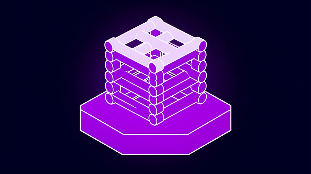
The learned part of the inspection system is only as good as the masks it was trained on, and the paper spends real effort on them. After manual curation, the labelled corpus holds 12,386 images from a first imaging campaign and 1,411 from a second campaign that expanded the helicoidal lattice, 13,797 in total. A third campaign, the large production cushion, was held out entirely for testing.
That total matters because LLNL’s announcement describes “a curated dataset of nearly 15,000 human-annotated images”. The paper’s own abstract says “≈13,800”, and its dataset table sums to 13,797, which is 1,203 images, or 8.7%, short of 15,000. It is a rounding choice rather than a flaw in the science, but it is the kind of detail worth checking before you quote a figure about any inspection system.
| Geometry | Campaign 1 | Campaign 2 | Total | Share | Test images |
|---|---|---|---|---|---|
| Face-centred tetragonal (FCT) | 8,018 | None | 8,018 | 58.1% | 802 |
| Helicoidal (HELI) | 2,833 | 1,411 | 4,244 | 30.8% | 424 |
| Simple cubic (SC) | 1,535 | None | 1,535 | 11.1% | 154 |
| Total | 12,386 | 1,411 | 13,797 | 100% | 1,380 |
The split was a stratified 80/10/10 into training, validation and test sets: 11,037 training images, 1,380 for validation and 1,380 for test. The imbalance is plain in the chart below, and the authors flag it as a limitation in their discussion.
Three lattices that look almost identical from above
The paper describes all three geometries as log-pile lattices built from layers that alternate by 90 degrees. They differ in how layers of the same orientation line up. In simple cubic, strands two layers apart sit directly above each other, leaving straight square channels. In face-centred tetragonal, alternate layers shift sideways by half a strand spacing, so each strand nests in the valley below it.
From a single top-down photograph, simple cubic and face-centred tetragonal look nearly the same: a row of parallel strands at equal spacing. What differs is how the lower layers show through. That is exactly the cue the inspection system must learn to see past, and it explains a result further down this section.
How the human labels were made
Masks were produced with Amazon SageMaker Ground Truth by a custom annotator pool. Each image was reviewed over two to three passes and accepted only when the labelled boundary sat within 3 pixels of the visible strand edge on each side. At 3.249 µm per pixel, that tolerance is about 9.7 µm per edge.
Annotators decided only which pixels belonged to the top layer. The scale came from the checkerboard, not from human judgement. The supplementary file lists 43 example masks shipped with the code, and the paper says the curated dataset and model weights are reachable through links in the repository documentation. That openness is rarer than it should be for training data in industrial vision work.
Leave one geometry out, and FCT falls hardest
To test generalisation, the team trained models that never saw one of the three geometries, then scored each on the geometry it had missed. The full model is flat across all three, scoring a Dice of 0.974 on simple cubic, 0.972 on FCT and 0.975 on helicoidal. The Dice coefficient measures overlap between predicted and human masks, where 1.0 is a perfect match.
Removing a geometry hurt most when that geometry was FCT, which fell to 0.831. The authors attribute this to corpus share rather than shape: FCT is about 58% of the labelled images and supplies most of the sub-surface variation the network learns from. A class-balanced sampler, which equalises how often each geometry is seen without discarding data, lifted the pooled test score to 0.980.
Why thresholds and edge detectors were not enough
The supplement benchmarks four classical segmenters from scikit-image, each tuned on the validation split and frozen before testing. None came close. The best, Otsu thresholding, reached a pooled Dice of 0.708, and Canny edge detection collapsed to 0.497 on the dense FCT lattice, where lower-layer bleed-through is worst.
| Method | Simple cubic | FCT | Helicoidal | All test images |
|---|---|---|---|---|
| Otsu thresholding | 0.705 | 0.699 | 0.727 | 0.708 |
| Sauvola adaptive thresholding | 0.702 | 0.620 | 0.726 | 0.662 |
| Canny edge detection | 0.674 | 0.497 | 0.711 | 0.582 |
| Frangi ridge filter | 0.651 | 0.620 | 0.656 | 0.634 |
| U-Net (LLNL) | 0.974 | 0.972 | 0.975 | 0.973 |
For anyone building a vision inspection system on a production line, this table is the case for a learned model in one glance. When the feature you care about looks like the background, rules tuned by hand plateau early, and no amount of threshold tweaking recovers the gap.
How Accurate Is the Inspection System Against Human Labels?
Segmentation scores say whether the mask looks right. The number a quality engineer cares about is whether the diameter is right. The paper tests that on 55 physical parts, using 283 held-out test images that were never used for training, with a median of five images per part and a range of one to 15.
The inspection system’s headline accuracy figures
Aggregated to one median per part, inspection system diameters track human-labelled diameters with a coefficient of determination (R²) of 0.824, a root mean square error (RMSE) of 3.40 µm, a mean absolute error of 2.92 µm and a mean absolute percentage error (MAPE) of 2.60%. The paper gives the tested range as roughly 240 to 290 µm. LLNL’s announcement summarises this as measurements “typically within a few micrometers of human-derived measurements”.
Two error numbers, two reference lines
The supplementary file adds a figure the press release does not mention. Measured against the identity line, where the inspection system’s value equals the human value, the raw part-level output has a residual RMSE of 7.48 µm and a mean bias of +5.98 µm, meaning the inspection system reads strands slightly wide on average. Applying the regression as a per-nozzle calibration removes the bias and brings RMSE down to 4.76 µm.
The paper does not explain why its main text reports 3.40 µm while the supplement reports 7.48 µm for the same 55 parts. One reading consistent with both figures is that 3.40 µm describes scatter around the fitted line, while 7.48 µm describes distance from the identity line. The MAPE supports that reading: 2.60% of a 250 µm strand is 6.5 µm, much closer to the uncalibrated figure.
A slope of 0.715 is a calibration problem, not a ceiling
The paper’s fitted line is predicted diameter = 0.715 × human diameter + 78.86 µm. A slope below 1 compresses the range. Solving the equation, the fit crosses the identity line at about 277 µm: below that the inspection system reads high, and above it low. For a 240 µm strand the fit predicts 250.5 µm, about 10.5 µm high. For a 290 µm strand it predicts 286.2 µm, about 3.8 µm low.
The authors call this “a systematic, correctable offset rather than an accuracy ceiling”, and the supplement’s calibration result backs that up. They also warn the regression describes one nozzle-and-ink regime and should not be extrapolated outside the tested diameter range. Image-level results, before aggregation across a part, are looser: an RMSE of 5.79 µm, a MAPE of 2.68% and an R² of 0.799 across the 283 images.
| Measure | Value | Level | Source |
|---|---|---|---|
| Pooled segmentation Dice | 0.973 | Image, 1,380 test images | Paper |
| R² | 0.824 | Part, 55 parts | Paper, Fig. 5 |
| RMSE | 3.40 µm | Part | Paper, Fig. 5 |
| Mean absolute error | 2.92 µm | Part | Paper, Fig. 5 |
| MAPE | 2.60% | Part | Paper, Fig. 5 |
| Fitted slope and intercept | 0.715 and 78.86 µm | Part | Paper, Fig. 5 |
| Raw RMSE against the identity line | 7.48 µm, mean bias +5.98 µm | Part | Supplement, Fig. S8 |
| RMSE after per-nozzle calibration | 4.76 µm, mean bias 0 | Part | Supplement, Fig. S8 |
| Image-level RMSE and MAPE | 5.79 µm and 2.68% | Image, 283 images | Supplement, Fig. S4 |
Is it precise enough for the job?
The useful test is whether the error is small relative to the problems the inspection system has to catch. The paper says its process-parameter perturbations changed filament diameter by about 10 to 20 µm. That is 2.9 to 5.9 times the 3.40 µm figure, 2.1 to 4.2 times the calibrated 4.76 µm, and 1.3 to 2.7 times the raw 7.48 µm. Calibrated, the margin is comfortable. Uncalibrated, a 10 µm shift sits close to the noise.
The 25 cm Cushion: Where the Inspection System Beats X-ray CT
The most striking demonstration is not a small test coupon but a production-scale cushion. LLNL printed a part with a designed footprint of 25 × 25 cm and ran the inspection system on it. For the second printed layer, the inspection system processed about 2,420 images and stitched the results into a map of filament diameter across the part.
How the inspection system mapped one layer from 2,420 images
The processed map covers a cropped interior of about 19 × 19 cm, deliberately excluding edge artefacts. That interior is 361 cm², or 57.8% of the 625 cm² designed footprint. Across it, the median predicted diameter was 253.4 µm, with a mean of 254.3 µm and a standard deviation of 6.7 µm. Outliers more than 2.5 standard deviations from their neighbours were removed before interpolation.
The image count is consistent with tiling that interior. Each 1,200-pixel frame covers about 3.9 × 3.9 mm, or 15.2 mm². Multiply by 2,420 and you get about 368 cm², within 2% of the 361 cm² interior. LLNL’s release rounds the count to “about 2,500 images”, and the paper’s abstract says “∼2.4k images per layer”.
The tilt the inspection system found and an average would have hidden
The map showed filament diameter drifting steadily from one side of the print bed to the other. The paper says this “strongly indicates a slight substrate tilt relative to the extrusion nozzle”. The supplement sketches the mechanism: with the nozzle travelling in a level plane over a slightly tilted build plate, the gap narrows on one side, squashing the strand into a wider line, and widens on the other, leaving a thinner one.
An average of 253.4 µm would have looked perfectly healthy. Only the spatial map exposed a hardware fault, diagnosed, in the authors’ words, “purely through software metrology”. It is the clearest argument in the paper for a per-layer inspection system rather than a single pass-or-fail number at the end. The supplement labels the tilt “suspected”, so treat it as a strong diagnosis rather than a measured angle.
Why X-ray CT could not inspect this part
X-ray CT gives full 3D structure, and the authors still call it the gold standard for cured geometry. The limit is scale. Useful CT metrology needs roughly ten voxels across a feature, so a 250 µm strand needs voxels of 25 µm or smaller. At that resolution the paper says CT is restricted to volumes on the order of 10 cm³, which “precludes whole-part analysis for cushions exceeding 50 cm³”.
The cushion’s thickness is not given, but the footprint settles the point: at just 1 mm thick, a 625 cm² part would be 62.5 cm³, already past the 50 cm³ line. A camera-based inspection system has no such ceiling, because it images one small tile at a time and stitches them together. The trade is depth. The camera sees only the top layer, as deposited, and cannot find voids buried inside a cured part. For background on the scanning side, industrial computed tomography is a good primer.
| Factor | On-machine camera (LLNL) | X-ray CT | Optical profilometry or structured light |
|---|---|---|---|
| When it runs | During printing, layer by layer | After printing and curing | Usually after printing |
| What it sees | Top-layer strand width, as deposited | Full 3D internal structure | Surface only |
| Part size limit | Grows with the number of images | About 10 cm³ at strand-scale resolution | Large areas, but slow |
| Material state | Uncured | Cured | Usually cured |
| Main weakness | No depth information | Volume against resolution trade-off | Performs poorly on translucent inks |
| Best use | Screening and spatial maps | Gold-standard verification | Surface checks |
Checking the Inspection System's "100,000 Times Faster" Claim
LLNL’s announcement says manually measuring a large image “could take a person from about 20 minutes to an hour”, and that the automated pipeline works “in milliseconds, or roughly 100,000 times faster on average than a human can”. The milliseconds are confirmed by the paper. The multiple is not something the paper states, so we ran the arithmetic on the figures it does publish.
What the paper actually timed for the inspection system
Inference plus post-processing averaged 57.1 ± 3.2 ms per image on a single NVIDIA A10G GPU, the accelerator used in Amazon EC2 G5 instances. The 2,420 images of the cushion layer took 2.3 minutes of GPU time. End to end, including stitching and file input and output, the layer took about 15.2 minutes. The paper reports no human timing at all.
The arithmetic against a 20-to-60-minute human
Twenty minutes is 1,200,000 ms. Divided by 57.1 ms, that is about 21,000 times faster. Sixty minutes gives about 63,000 times. For the inspection system to be 100,000 times faster at 57.1 ms per image, a person would need about 95 minutes per image. Put the other way, at 20 to 60 minutes per image, the inspection system would need 12 to 36 ms per image.
LLNL may have timed a different step, image size or machine from the one the paper reports, and “a large image” in the release may not mean one 1,200-pixel frame. The published figures support “tens of thousands of times faster” per image. That is still an enormous gain for any inspection system, and it does not need rounding up.
What one layer would cost a person
The per-layer view is more practical. At 20 to 60 minutes per image, a person measuring all 2,420 images of one cushion layer would need 807 to 2,420 hours, which is 108 to 323 working days at 7.5 hours a day. The inspection system does it in about 15.2 minutes end to end, a speed-up of roughly 3,200 to 9,600 times once stitching and file handling are counted.
| Item | Figure | Source or arithmetic |
|---|---|---|
| Inference and post-processing per image | 57.1 ± 3.2 ms | Paper |
| GPU time for one 2,420-image layer | 2.3 minutes | Paper; 2,420 × 57.1 ms = 138 seconds |
| End-to-end time for that layer | About 15.2 minutes | Paper |
| Human time per large image | 20 to 60 minutes | LLNL release only |
| Human time for one layer | 807 to 2,420 hours | 2,420 images × 20 or 60 minutes |
| Speed-up per image | About 21,000× to 63,000× | 20 or 60 minutes ÷ 57.1 ms |
| Speed-up for the whole layer | About 3,200× to 9,600× | Human hours ÷ 15.2 minutes |
| Speed-up claimed | “Roughly 100,000 times” | LLNL release only |
LLNL's Press Release vs the Paper: An Inspection System Claims Ledger
Press releases compress, and research laboratories are no exception. The ledger below lines up each specific claim in LLNL’s announcement against the peer-reviewed paper and its supplement. Most claims hold. A few are rounded in the flattering direction, and two describe ambitions for the inspection system rather than results.
| Claim | LLNL release, 14 Sep | Paper and supplement | Verdict |
|---|---|---|---|
| Labelled images | “Nearly 15,000” | 13,797, or “≈13,800” in the abstract | Rounded up by 8.7% |
| Images for one large layer | “About 2,500” | About 2,420 | Rounded up |
| Cushion size | About 25 by 25 cm | Designed 25 × 25 cm; map covers about 19 × 19 cm | Accurate for the print |
| Parts tested | 55 parts | 55 parts, 283 test images | Confirmed |
| Accuracy | “Typically within a few micrometers” | RMSE 3.40 µm; raw 7.48 µm against identity, 4.76 µm calibrated | Fair once calibrated |
| Speed | “In milliseconds” | 57.1 ms per image on one A10G GPU | Confirmed |
| Speed multiple | “Roughly 100,000 times faster” | Not stated; published figures imply about 21,000× to 63,000× | Not supported by the paper |
| Human measuring time | 20 minutes to an hour per large image | Not reported | Release only |
| Build plate tilt | Pattern “pointed to a slight tilt” | “Strongly indicates”; supplement says “suspected” | Release slightly firmer |
| Other processes | Adaptable to other additive and subtractive manufacturing | “Demonstrated on a single platform”; not validated elsewhere | Intent, not result |
| Autonomy | Accept or reject calls, digital twins | Closed-loop control “beyond the scope of this work” | Future goal |
| Openness | Not mentioned | Code on GitHub; dataset and weights linked from it | Paper goes further |
Where the release rounds up
The dataset size, the per-layer image count and the speed multiple all move in the same direction: bigger. None of them changes the scientific conclusion, and “nearly 15,000” and “about 2,500” are defensible as loose rounding. The 100,000× figure is different in kind, because it cannot be reproduced from anything the paper publishes.
Where the paper is more careful than the headline
The paper repeatedly limits its own claims. It says the workflow was “demonstrated on a single platform”, that the software has not been validated on other systems, that closed-loop control is out of scope, and that the tilt is an indication rather than a direct measurement. That caution is a good sign for the research, and a reason to read the paper before building plans on the release.
What neither document settles
Neither document reports how the inspection system performs on a different ink, printer or camera, how often the model must be retrained as materials change, or what the whole setup costs to build and run. Neither compares camera measurements with CT on the same cured part; the paper argues that would measure print-to-cure change rather than validate the inspection system, and lists it as future work.
What the Inspection System Does Not Do Yet
The paper’s discussion section is unusually frank about limits. For anyone tempted to treat the announcement as a finished product, these are the gaps to keep in mind before planning around the inspection system.
One printer, one camera, one ink family
Every result comes from a single DIW platform with one optical configuration and one siloxane ink family. The authors say transfer “to different hardware, optics, or inks will require per-system tuning of illumination, focus, and calibration”. A more translucent or differently pigmented ink would reduce the contrast between the top layer and the layers below, degrading segmentation until the model is fine-tuned on new labels.
It measures, but it does not yet control or decide
The inspection system produces a measurement stream. It does not adjust the printer, and it does not reject parts automatically. The paper positions its per-layer data as “a necessary building block” toward closed-loop control. Weston looks further ahead: “When the printer can inspect its own work, we can start thinking about the system making its own accept/reject calls.”
New conditions mean new labels
Creating high-quality masks at scale is, in the authors’ words, “time and resource intensive” and “a practical bottleneck” for new inks, optics or lattice families. Data collection and model maintenance are currently manual. They suggest active learning or human-in-the-loop frame selection to reduce the annotation burden and to catch model drift over time.
Uncured width is not cured geometry
Because the camera measures uncured strands, its numbers are not the dimensions of the finished part. Cure shrinkage of about 2%, gravitational settling and the elliptical cross-section of cured strands each introduce differences of the same order as the reported error. CT stays necessary wherever cured 3D geometry is the specification.
| Limitation | What the paper says | Practical consequence |
|---|---|---|
| Single platform | “Demonstrated on a single platform” | Budget for re-tuning on your own hardware |
| Ink dependence | Translucent inks reduce contrast | Expect new labels for new materials |
| Dataset imbalance | FCT is about 58% of the corpus | Weaker on under-represented geometries |
| Proportional bias | Slope of 0.715 before calibration | Calibrate per nozzle before trusting absolute values |
| No closed loop | Control is outside the paper’s scope | A person still acts on the data |
| Manual upkeep | Data collection and model maintenance are manual | Plan ongoing labelling effort |
Where This Inspection System Fits in AI Quality Control for Additive Manufacturing
Machine learning has been applied to in-situ monitoring in additive manufacturing for years, so the novelty here is specific. The paper’s argument is that most prior work classifies defects rather than measuring geometry, and that where geometry has been measured, it has been one strand or one layer at a time.
| Approach in prior work | Typical process | Output |
|---|---|---|
| Deep models for melt-pool, porosity and anomaly monitoring | Metal powder bed, directed energy deposition | Defect detection and prediction |
| Object detection and convolutional classifiers | Polymer extrusion | Classes such as warping, delamination, stringing and over- or under-extrusion |
| Multi-modal optical monitoring | Extrusion | Spatial artefact maps and closed-loop control |
| Semantic segmentation of AM images | Various | Porosity or structural regions for failure analysis |
| Vision and ML width measurement | Fused filament fabrication | Extrusion width to about 90 µm over 2D patterns |
| Classical machine vision contour matching | DIW | Single-layer dimensional accuracy |
| ML-enhanced in-situ rheology | DIW | Ink properties, not part geometry |
| LLNL on-machine inspection system | DIW lattices | Calibrated strand diameter per layer and full-part maps |
From spotting defects to measuring geometry
The paper claims, “to our knowledge”, the first practical, non-destructive, full-part, per-layer geometric metrology during DIW. That is a narrower claim than “AI inspects 3D prints”, which many products already do. The difference is the output. A defect classifier says “stringing here”. This inspection system says “this region of the layer runs wider than the rest”, which is a number a process engineer can act on.
Kansas City, digital twins and accept-or-reject calls
Weston said the capability is expected to move to Kansas City for evaluation on production-relevant systems and components. The release calls the site the Kansas City National Security Complex; its own website uses the name Kansas City National Security Campus, managed by Honeywell Federal Manufacturing & Technologies for the National Nuclear Security Administration, with nearly 7,000 people working there.
Longer term, Weston said inspection data could feed simulations and digital twins that link a part’s measured structure to its predicted performance, potentially speeding acceptance and qualification. Our overview of digital twins for UK manufacturers explains why that link between measured and modelled parts is where the value tends to sit.
Why a national lab’s cushion matters beyond defence
Giera said the approach was developed to be adaptable to other additive technologies, conventional subtractive manufacturing and experimental systems at the Lab. The paper has not shown that yet, but the pattern is general: a calibrated camera, a small learned model for the hard perceptual step, and deterministic measurement code. It applies to extrusion, dispensing, coating and many other processes where geometry decides quality. For the business case around that kind of project, see our piece on data and AI in manufacturing.
What Manufacturers Can Borrow From the Inspection System
Few manufacturers print siloxane lattices, but many are exploring camera-based checks on their lines. The LLNL work is a useful template precisely because it is careful about measurement rather than impressive about AI. These are the design decisions worth copying into your own inspection system.
Define the measurand before choosing a model
LLNL decided first what number it needed, the width of the newest strand at the moment of deposition, and designed the optics around it. Many computer vision projects start with a model and go looking for a use. Starting from the measurement also tells you what the camera cannot see, which in this case is everything below the top layer.
Calibrate the inspection system to a physical standard
The pixel pitch was verified against a checkerboard target with about 1 µm positional accuracy, and the telecentric lens removed working-distance errors. That turns a model’s output into a traceable measurement. If your inspection system cannot say how many micrometres a pixel represents, and prove it, it is estimating rather than measuring.
Budget for labelling like a capital cost
The 13,797 masks were each reviewed in two to three passes, and the paper treats that corpus as a core asset. Our look at annotation errors in object detection datasets shows how quietly bad labels degrade results. Plan labelling time, quality checks and relabelling for every new material or camera before the project starts.
Give the inspection system a human reference and a bias check
LLNL measures accuracy against human-labelled masks, and the supplement exposes a correctable proportional bias. Any production deployment should keep a small, regularly refreshed human-measured reference set and re-check the calibration line on a schedule. That is the same discipline good predictive analytics teams apply to any model that drifts.
Start from the open code, carefully
The llnl/diw-strand-metrology repository on GitHub contains training code, SageMaker notebooks, a distance-transform and skeletonisation demo, the classical baseline and sample masks. When we checked on 15 September 2026, GitHub’s API detected no licence file for the repository, so confirm reuse terms with LLNL before building a commercial inspection system on it.
| Decision | LLNL’s choice | Question for your line |
|---|---|---|
| Measurand | Uncured top-layer strand width | What single number decides pass or fail? |
| Optics | Telecentric 2× objective and LED ring | Does magnification change as parts or conveyors move? |
| Scale | 3.249 µm per pixel, checkerboard-verified | Can you prove the pixel size? |
| Model scope | U-Net for segmentation only | Which step genuinely needs a learned model? |
| Measurement | Distance transform and skeleton, deterministic | Can an auditor follow the measurement code? |
| Labels | 13,797 masks, two to three review passes | Who labels, how often, and at what cost? |
| Reference | Human-labelled parts and per-nozzle calibration | How will you detect bias drift? |
| Compute | Single A10G GPU, 57.1 ms per image | Edge device or cloud, and what latency? |
If you are scoping a similar project, our data science services and IoT solutions teams work on sensor and camera data pipelines, and our guide to IT support for manufacturing companies covers the infrastructure around them. For the strategic framing, see AI strategy and our Industry 4.0 guide.
Inspection System FAQ
What is LLNL’s AI-powered inspection system?
It is a camera-and-software pipeline mounted on a direct ink writing 3D printer at Lawrence Livermore National Laboratory. A camera photographs every printed layer, a U-Net model identifies the newest strands, and classical image processing measures their diameter, producing per-part statistics and full-layer maps.
How accurate is the inspection system?
Against human-labelled measurements on 55 parts, the paper reports an RMSE of 3.40 µm and a MAPE of 2.60% for strands of roughly 240 to 290 µm. The supplement shows a raw error of 7.48 µm against the identity line, falling to 4.76 µm after per-nozzle calibration.
Is it really 100,000 times faster than a person?
The paper reports 57.1 ms per image but no human timing. Using the release’s estimate of 20 to 60 minutes for a person, that is about 21,000 to 63,000 times faster per image. The 100,000 figure appears only in the press release.
Does the inspection system replace X-ray CT?
No. It screens parts during printing and maps large layers that CT cannot cover at strand-scale resolution, but it sees only the uncured top layer. CT remains the reference for cured 3D geometry and for defects hidden inside a finished part.
Which 3D printing processes does it work with?
So far, only direct ink writing of siloxane lattices on one LLNL printer. LLNL says the approach is designed to be adaptable to other additive and subtractive processes, but the paper has not validated that, and the authors expect per-system tuning.
Can I download the code behind the inspection system?
Yes. The code is public on GitHub at llnl/diw-strand-metrology, and the paper says the dataset and model weights are linked from its documentation. GitHub detected no licence file when we checked, so confirm reuse terms before any commercial use.
References
LLNL: AI-powered inspection system gives 3D printers ‘a brain behind the eyes’
GitHub: llnl/diw-strand-metrology
arXiv: U-Net: Convolutional Networks for Biomedical Image Segmentation
Kansas City National Security Campus
LLNL: Advanced Materials and Manufacturing
LLNL Laboratory Directed Research and Development
Wikipedia: Industrial computed tomography
More AI coverage: explore Progressive Robot's AI Models, Tools & Releases hub — hands-on reviews, setup guides and benchmarks in one place.